Every parameter and its default
The complete input reference — every card on the five stage tabs, each field's shipped default, its accepted range, and what it changes.
Every input ships with a working default, so a first run needs none of them changed. Select a boundary file, click Generate Layout, and the plant is built from the values on this page. The boundary file is the only input with no default — see Boundary files.
The inputs sit on five stage tabs under the pinned Generate Layout button: Site · Array · Electrical · Yield · Tools. Every card on a tab is a collapsible group, expanded by default. Two things change what you see: the mounting type decides which array cards appear, and the inverter topology retitles the inverter card and relabels several rows. Both are chosen at launch; the ribbon's design chip ("Fixed tilt · String inverter ▾") opens another window for a different combination — see Choosing a design mode and The main window.
The tables below are in tab order, then card order, and the rows within each table follow the order of the fields on screen.
The five tabs
| Tab | Cards, in order | Changes with the design |
|---|---|---|
| Site | Input Boundary File · Site Parameters · Structures & Shadow (keep-clear) · Topography (slope-aware exclusion) | — |
| Array | MOUNTING chip · Module Specifications · MMS-Table Configuration · Spacing & Tilt | A tracker design replaces the last two with a single Tracker Configuration card |
| Electrical | String Inverter · Cables | A central design retitles the first card SMB – String Monitoring Box and adds one field |
| Yield | Run Energy Calculation · Energy Yield | Two loss labels follow the topology |
| Tools | Obstructions · Main Control Room & Objects · Studies | Locked until a layout exists |
Site tab
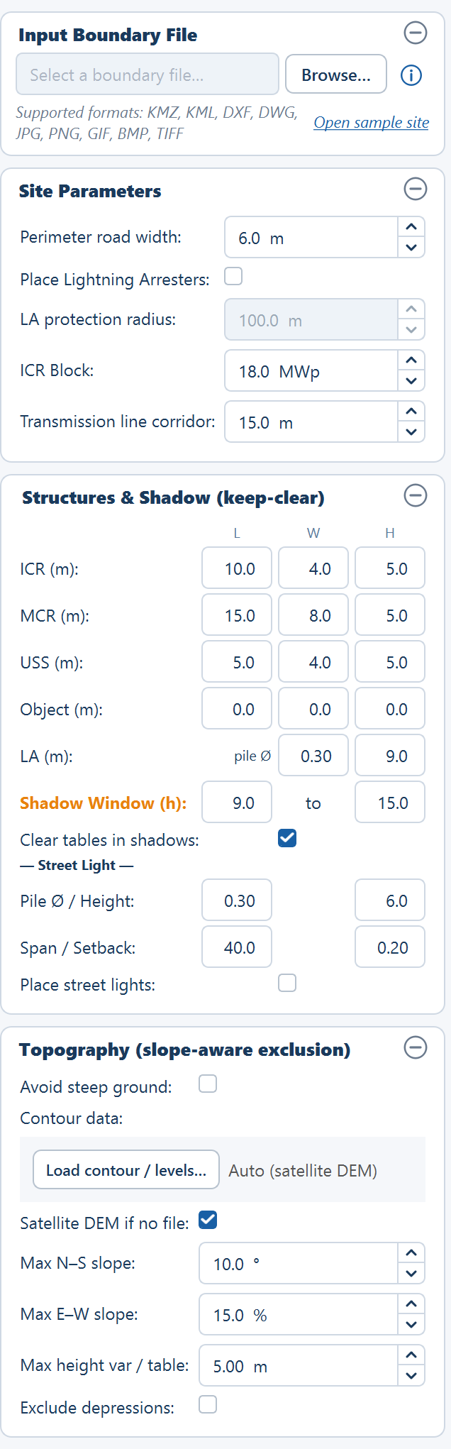
Input Boundary File
A read-only path field with the placeholder "Select a boundary file…", a Browse… button, and a round ⓘ button that opens the KMZ File Preparation Guide. Under the field a line reads "Supported formats: KMZ, KML, DXF, DWG, JPG, PNG, GIF, BMP, TIFF"; while the field is empty an Open sample site link beside it loads the bundled sample — one boundary with a pond, a transmission line and an obstruction. Once a file is read that line becomes the boundary summary, for example "1 boundary · 1 obstacle · 1 line obstruction".
| Field | Default | Range | What it does |
|---|---|---|---|
| Browse… | empty | .kmz .kml .dxf .dwg .jpg .jpeg .png .gif .bmp .tif .tiff | Chooses the file the plant boundary is read from. A CAD drawing or an image also opens the Site reference window for the site's coordinates. |
In depth: Boundary files, CAD drawing and Image boundary.
Site Parameters
These settings decide how much ground is available before a single table is placed, and how much equipment goes on what remains. In depth: Site parameters.
| Field | Default | Range | What it does |
|---|---|---|---|
| Perimeter road width | 6.0 m | 0.0–50.0 m | Shrinks the plant boundary inward by this distance to give the usable area. Nothing is placed in the band left behind. |
| Place Lightning Arresters | off | — | On, arresters are placed on a coverage grid and the tables they overlap are cleared. Off, tables fill the whole usable area; arresters can still be added by hand in Sketch Mode. |
| LA protection radius | 100.0 m | 10.0–500.0 m | The radius one arrester is taken to protect, and the spacing of the grid they sit on. Enabled only when arresters are on. |
| ICR Block | 18.0 MWp | 0.1–500.0 MWp | The DC capacity one inverter control room serves. The room count is the plant capacity divided by this, rounded up. |
| Transmission line corridor | 15.0 m per side | 0.0–500.0 m | The setback applied to each side of every line feature that is not a road, so the cleared strip is twice this figure — 30 m at the default. A road line takes half its own width each side instead. |
The corridor tooltip recommends raising the setback for higher-voltage lines, for example 30 m per side for a 400 kV line.
Structures & Shadow (keep-clear)
A grid with the column headers L, W and H: Length (E-W) × Width (N-S), plus a Height that drives the shadow footprint. The compact fields carry no unit; the row labels do ("ICR (m):"). In depth: Structures and shadow.
| Field | Default | Range | What it does |
|---|---|---|---|
| ICR — L / W / H | 10.0 / 4.0 / 5.0 m | 0.0–500.0 / 0.0–500.0 / 0.0–200.0 m | The inverter control room building. The layout clears every table overlapping this footprint. |
| MCR — L / W / H | 15.0 / 8.0 / 5.0 m | 0.0–500.0 / 0.0–500.0 / 0.0–200.0 m | The main control room, placed by hand once per site. |
| USS — L / W / H | 5.0 / 4.0 / 5.0 m | 0.0–500.0 / 0.0–500.0 / 0.0–200.0 m | The unit substation dropped in every plot that does not hold the MCR, on a multi-plot site. |
| Object — L / W / H | 0.0 / 0.0 / 0.0 m | 0.0–500.0 / 0.0–500.0 / 0.0–200.0 m | A generic structure you place yourself. A height of 0 means not configured. |
| LA (m) — pile Ø | 0.30 m | 0.0–5.0 m | Nothing. A recorded figure only — it reaches no placement, no quantity and no export. |
| LA (m) — height | 9.0 m | 0.0–100.0 m | Nothing. A recorded figure only — it casts no shadow and reaches no output. |
| Shadow Window (h) | 9.0 to 15.0 | 4–12 / 12–20 solar hours | The solar-time window the keep-clear sweeps on every day of the year. A later end adds the low-sun afternoon tail and roughly doubles the ground each 5 m building sterilises. |
| Clear tables in shadows | on | — | Removes tables and tracker units falling inside the year-round shadow footprint of the ICR, MCR and objects during the window. Arresters are not in that list. |
| Street Light — Pile Ø / Height | 0.30 / 6.0 m | 0.0–5.0 / 0.0–50.0 m | Pole foundation diameter, and the pole height its shadow is cast from. |
| Street Light — Span / Setback | 40.0 / 0.20 m | 1.0–500.0 / 0.0–50.0 m | Pole-to-pole spacing along the perimeter, and how far inside the fence the poles are inset. The count is roughly the perimeter divided by the span. |
| Place street lights | off | — | On, poles are placed along the perimeter and the tables their shadow touches are cleared. |
Every length and width accepts 0.0–500.0 m and every height 0.0–200.0 m, to one decimal place, and the ranges are the same for all four structures. The two arrester fields are the exception in the card: they accept a value and then feed nothing at all, not even the project file.
On a multi-plot site, Place MCR drops a USS of the size above into every plot except the one holding the MCR, and each plot's control rooms route their medium-voltage cables to their own USS. The USS-to-MCR link itself is an overhead line or a buried cable handled outside the automatic routing.
Topography (slope-aware exclusion)
Does nothing until enabled. In depth: Topography.
| Field | Default | Range | What it does |
|---|---|---|---|
| Avoid steep ground | off | — | Enables the whole card. Off, no terrain exclusion is applied. |
| Contour data | "Auto (satellite DEM)" | — | The Load contour / levels… button accepts a DXF contour file in the project's UTM coordinates, or a CSV of longitude, latitude and elevation. The file dialog accepts .dxf, .dwg, .csv and .txt. |
| Satellite DEM if no file | on | — | Builds the elevation model from public satellite elevation data when no contour file is supplied. Needs an internet connection. |
| Max N–S slope | 10.0° | 0.0–45.0° | Ground steeper than this across the rows is excluded. |
| Max E–W slope | 15.0 % | 0.0–100.0 % | Ground steeper than this along the rows is excluded. |
| Max height var / table | 5.0 m | 0.0–30.0 m | The ground relief allowed within one table footprint — the pile-reveal differential. |
| Exclude depressions | off | — | On, hollows where water would pool are excluded as well as steep ground. |
Any terrain failure — no network, an unreadable file — is non-fatal: the layout proceeds without terrain exclusion. Contours draw green for low ground through blue to red for high, switched on by the Contour / terrain row of the Layers ▾ popover, and the excluded area is reported in acres.
Array tab
The tab opens with a read-only MOUNTING chip — "Fixed-tilt MMS tables" or "Single-axis tracker" — that records the choice made at launch.
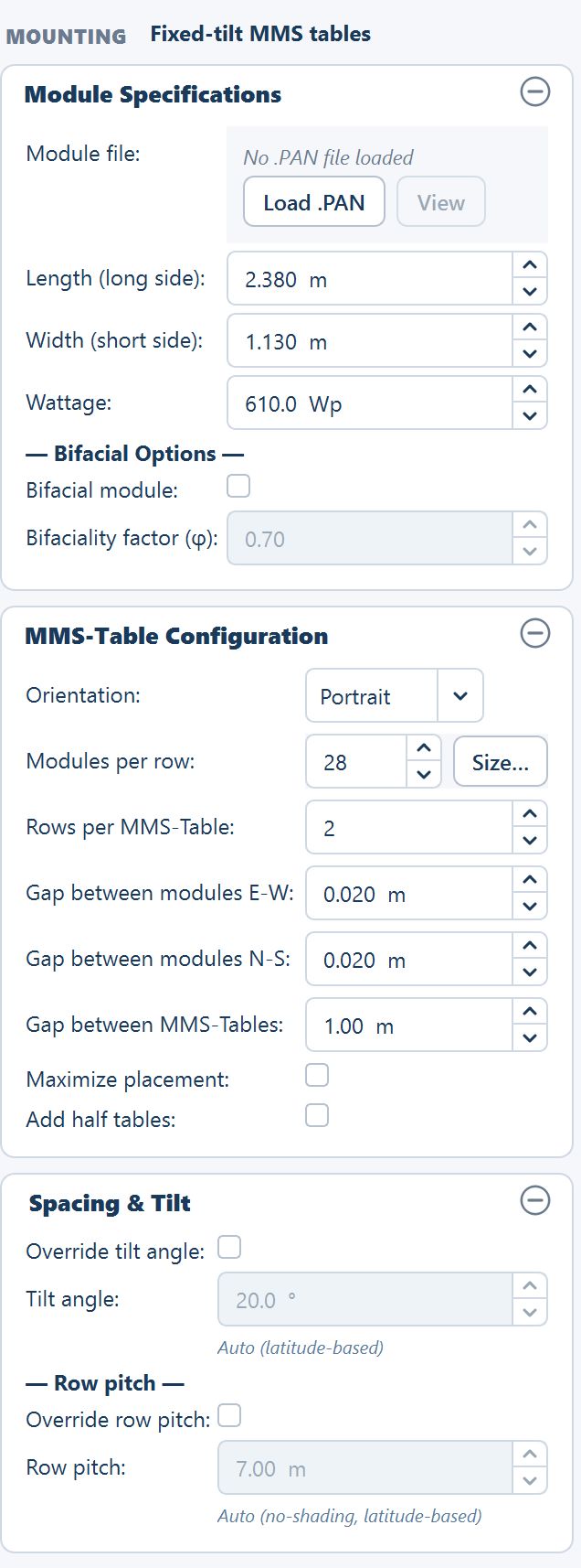
Module Specifications
Shown in both designs. In depth: Module specifications.
| Field | Default | Range | What it does |
|---|---|---|---|
| Module file | "No .PAN file loaded" | — | Load .PAN reads a PVsyst module file; View opens it read-only once loaded. |
| Length (long side) | 2.38 m | 0.5–5.0 m | The module's long edge. On fixed tilt it runs north–south in Portrait and east–west in Landscape. |
| Width (short side) | 1.13 m | 0.5–3.0 m | The module's short edge. On fixed tilt it runs east–west in Portrait and north–south in Landscape. |
| Wattage | 610 Wp | 100–1000 Wp | Nameplate DC power of one module. Plant DC capacity is this multiplied by the placed module count. |
| Bifacial module | off | — | Enables the rear-side gain model and unlocks the bifaciality factor. |
| Bifaciality factor (φ) | 0.70 | 0.50–0.95 | Rear-side efficiency as a fraction of the front. Enabled only when Bifacial module is on. |
- Load .PAN fills in the wattage, the long side and the short side. When the file declares a bifacial module it also ticks Bifacial module and fills φ, and it recomputes the temperature loss. Dimensions are accepted in metres or in millimetres. The file row then shows the module label in green.
- View opens the read-only viewer with the tabs Basic data, Sizes and technology, Model parameters, Additional data and Graphs.
- Loading a module file asks nothing. String sizing is opened from the Size… button beside Modules per row (fixed tilt) or Modules per string (N–S) (tracker) — see String sizing and the string-sizing fields below.
The bifaciality tooltip gives a typical φ of 0.65–0.80 and a typical bifacial energy gain of 5–15 % over a monofacial module.
MMS-Table Configuration
Fixed tilt only. In depth: Table configuration.
| Field | Default | Range | What it does |
|---|---|---|---|
| Orientation | Portrait | Portrait or Landscape | Decides which module edge runs east–west and which runs north–south. |
| Modules per row (with Size…) | 28 | 1–100 | Modules side by side along one row of the table, east to west. |
| Rows per MMS-Table | 2 | 1–10 | Rows of modules stacked up the tilted face. One row is one string. |
| Gap between modules E-W | 0.020 m | 0.0–5.0 m | Clear space between neighbouring modules within a row. |
| Gap between modules N-S | 0.020 m | 0.0–5.0 m | Clear space between the stacked rows on one table. |
| Gap between MMS-Tables | 1.0 m | 0.0–20.0 m | Clear space between one table and the next in the same row — east–west only; north–south spacing is the row pitch. Also the span of a standard inter-table bridge when a cleaning fleet is sized. |
| Maximize placement | off | — | Positions each row of tables independently to hug the exact boundary edge. Table columns are no longer aligned across rows, and generation takes longer on a large site. |
| Add half tables | off | — | Allows a half-width table, carrying half the strings, wherever a full table will not fit. Half tables are also available in Sketch Mode. |
Table dimensions follow from the counts and the gaps:
table width  = modules per row × module E-W dimension
             + (modules per row − 1) × gap between modules E-W

table height = rows per table × module N-S dimension
             + (rows per table − 1) × gap between modules N-S
Both options at the bottom of the card are covered together on Maximize placement and half tables.
Spacing & Tilt
Fixed tilt only. Both values are derived from the site latitude unless you override them. In depth: Spacing and tilt.
| Field | Default | Range | What it does |
|---|---|---|---|
| Override tilt angle | off — the line under it reads "Auto (latitude-based)" | — | Off, the tilt is derived from the site latitude. On, your value is used. |
| Tilt angle | 20.0° | 0.0–90.0° | The fixed angle of the module plane. Enabled only when the override is on. |
| Override row pitch | off — "Auto (no-shading, latitude-based)" | — | Off, the pitch is the no-shading pitch at winter-solstice solar noon. On, your value is used. |
| Row pitch | 7.0 m | 1.0–50.0 m | Centre-to-centre spacing between rows of tables. Enabled only when the override is on. |
The automatic rules, both shown in the card's own tooltips:
tilt  ≈ latitude × 0.76 + 3.1°
pitch = L·cos(tilt) + L·sin(tilt) / tan(solar elevation)
L is the table height in the tilt plane. After a layout runs, the derived
values are reported inline — "Auto → 12.3° (latitude-based)",
"Auto → 7.42 m (no-shading, latitude-based)" — and pre-filled into the
still-greyed-out boxes so you can start from them. Reported GCR is the
table height divided by the row pitch.
Tracker Configuration
Tracker only. This one card replaces both the table card and the spacing card; its sections are Tracker Geometry, Row Spacing and Tracker Parameters. In depth: Tracker configuration.
| Field | Default | Range | What it does |
|---|---|---|---|
| No. of strings per tracker | 2 | 1–20 | Strings carried end to end along one tracker unit. |
| Modules across tracker (E–W) | 1 | 1–8 | Modules side by side across the torque tube. Sets the aperture. |
| Module orientation | P config (Portrait) | P or L config | P config puts the module long side east–west. L config (Landscape) puts the long edge north–south along the torque tube. |
| Modules per string (N–S) (with Size…) | 28 | 4–120 | Modules in series along the tube per string. The tooltip gives a typical range of 14–30. |
| Gap between modules E–W | 0.020 m | 0.0–5.0 m | Clear space between modules across the tube. |
| Gap between modules N–S | 0.020 m | 0.0–5.0 m | Clear space between modules along the tube. |
| Tracker E-W pitch | 5.5 m | 1.0–30.0 m | Centre-to-centre spacing between tracker columns. Divides into the aperture to give GCR. The tooltip gives a typical range of 4.5–7 m. |
| N–S service gap between units | 2.0 m | 0.0–20.0 m | Clear space between one tracker unit and the next along the same column. |
| Max rotation angle (±) | 55.0° | 5.0–75.0° | The rotation limit either side of horizontal. A reference and shading-analysis input. |
| Tracker height from ground | 1.5 m | 0.5–10.0 m | Torque-tube height. A reference and shading-analysis input. |
| Maximize placement | off | — | Positions each column independently to hug the boundary edge. |
| Add half trackers | off | — | Allows a half-length unit wherever a full one will not fit. |
The unit dimensions as placed:
n along tube    = strings per tracker × modules per string
aperture (E-W)  = modules across × module E-W dimension
                + (modules across − 1) × gap between modules E–W
length (N-S)    = n along tube × module N-S dimension
                + (n along tube − 1) × gap between modules N–S
modules/tracker = modules across × strings per tracker × modules per string
N-S step        = length + N–S service gap
A green preview line under the card reports Aperture (E-W), Length (N-S), GCR and Modules/tracker as you type. Treat it as indicative: it leaves the module gaps out of the first two, so on the shipped defaults the previewed length is 1.10 m short of the placed one.
The east–west pitch has a silent floor. A pitch at or below the aperture is raised to the aperture plus 0.5 m without a warning, and the reported GCR uses that effective pitch.
Electrical tab
String Inverter, or SMB – String Monitoring Box
The card title and the row labels follow the topology: String Inverter in a string design, SMB – String Monitoring Box in a central design. In depth: Inverters.
| Field | Default | Range | What it does |
|---|---|---|---|
| Max strings per inverter (string) / Max strings per SMB (central) | 20 | 1–500 | How many strings one inverter or one string monitoring box accepts. One string is one row of modules within an MMS-Table. |
| Max SMB per Central Inverter (central only) | 10 | 1–200 | How many boxes feed one central inverter. The central inverter's capacity is the box capacity multiplied by this. |
| OND (inverter) | "No OND file loaded" | — | Load .OND reads a PVsyst inverter file; View opens it read-only once loaded. |
- Load .OND shows the manufacturer and model on the row. Its PmaxOut figure drives the plant AC capacity, falling back to Pnom when absent. Loading it does not set the inverter efficiency on the Yield tab.
- View opens the read-only viewer with the tabs Main parameters, Efficiency curve, Additional parameters, Output parameters and Sizes and technology.
- In a central design a maximum of 4 central inverters are housed in one control room building.
Cables
In depth: Cable options.
| Field | Default | Range | What it does |
|---|---|---|---|
| Calculate cables | off | — | Routes and measures the string DC cables and the AC cables (or the DC trunks to the central inverter, counted twice for the two conductors). Off, the inverter and box counts are still computed and every cable row reads —. |
| Inter-module lead | 0.5 m/module | 0.0–2.0 m/module | Inter-module string cable per module, counted once per string. Fixed-tilt tables only. |
| String return run along table | on | — | One conductor runs back along the table so both leads exit beside each other. Untick for U-wired strings whose leads exit the same end. Fixed-tilt tables only. |
| DC cable slack | 10.0 % | 0.0–30.0 % | Slack and wastage added to the DC string-cable total. |
Ticking Calculate cables raises Cable Calculation — Performance Notice: cable calculation can take a long time on large or complex layouts. The buttons are Enable Now and Not Now (Recommended), and the recommendation is the default: generate the layout first without cables, review it, then enable them for the final run. Reopening a project does not raise it.
Yield tab
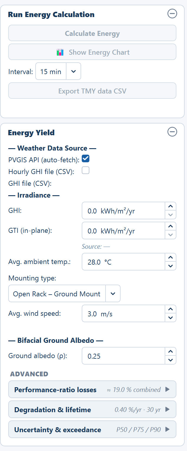
Run Energy Calculation
Not inputs, but the card the tab opens with: Calculate Energy, 📊 Show Energy Chart, an Interval: selector (1 min, 10 min, 15 min, 30 min, 1 hour) for the time-series export, Export TMY data CSV, and a status line. All are disabled until a layout exists. In depth: How yield is calculated and Time series.
Energy Yield
Nothing here affects where a table goes — it decides what the placed plant is predicted to generate.
Weather Data Source
Two mutually exclusive tick boxes. In depth: Weather data.
| Option | Default | What it does |
|---|---|---|
| PVGIS API (auto-fetch) | selected | Fetches irradiance for the site from the EU Joint Research Centre service when you calculate energy. No key or account. Falls back to NASA POWER where PVGIS has no data. |
| Hourly GHI file (CSV) | — | Reveals a GHI file (CSV): row with Browse… for your own hourly weather file. |
Selecting the file option pops Hourly GHI File — Required Format: exactly 3 columns in order — an hourly timestamp, GHI in W/m², and ambient temperature in °C. A full year is 8 760 rows, and a header row is optional and detected automatically. The application accepts more than that reminder suggests — column names are matched flexibly, and an in-plane irradiance column is accepted as well:
| Quantity | Accepted column names |
|---|---|
| Time | time, datetime, date, timestamp, time(utc), time(local), date/time |
| GHI | ghi, g(h), gh, global_horizontal, global horizontal irradiance, irradiance, solar irradiance, allsky_sfc_sw_dwn |
| GTI | gti, g(i), gi, in-plane irradiance |
When the file carries a temperature column, monthly average temperatures come from the file instead of from the seasonal model.
Irradiance and site conditions
| Field | Default | Range | What it does |
|---|---|---|---|
| GHI | 0.0 kWh/m²/yr | 0–3000 kWh/m²/yr | Annual global horizontal irradiance. Filled automatically once weather data is fetched or read. |
| GTI (in-plane) | 0.0 kWh/m²/yr | 0–3500 kWh/m²/yr | Annual irradiance on the tilted module plane. Filled automatically, and the figure the yield is built from. |
| (source line) | "Source: —" | — | Reads "Source: PVGIS (EU JRC) — auto fetched", "Source: NASA POWER — auto fetched" or, in red, "Source: Auto-fetch failed — switch to GHI file". |
| Avg. ambient temp. | 28.0 °C | −10–55 °C | Site air temperature used by the module temperature model. |
| Mounting type | Open Rack – Ground Mount | 4 options | Selects the Sandia thermal coefficient pair below. |
| Avg. wind speed | 3.0 m/s | 0.5–15.0 m/s | Site wind speed used by the module temperature model. |
| Ground albedo (ρ) | 0.25 | 0.05–0.80 | Reflectance of the ground. It feeds only the rear-side gain of a bifacial module; it has no effect on a monofacial one. See Bifacial gain. |
The four mounting configurations and their coefficient pairs:
| Mounting type | a | b |
|---|---|---|
| Open Rack – Ground Mount | −3.56 | −0.075 |
| Roof Mount – Close | −2.81 | −0.0455 |
| Stand-off Mount | −3.23 | −0.130 |
| Insulated Back | −2.81 | −0.0455 |
They feed the module temperature, and through it the temperature loss:
T_module = T_ambient + G × exp(a + b × W)
Loss (%) = |μPmpp| × (T_module − 25)
W is the wind speed and μPmpp is the module's power temperature coefficient,
read from the module file. G is the average operating irradiance derived from
GTI as the smaller of 900 W/m² and GTI × 1000 / (365 × 8), or 600 W/m² when
GTI is still 0. Once a module file is loaded a formula trace under the wind
speed shows the working. See Temperature losses.
ADVANCED expanders
Three expanders, collapsed by default, each header carrying a live summary.
Performance-ratio losses (summary "≈ 19.0 % combined" on the defaults). Every loss is a percentage, and together they give the performance ratio the yield is multiplied by. In depth: Losses and performance ratio.
| Field | Default | Range | What it does |
|---|---|---|---|
| String Inverter efficiency (string) / Central Inverter efficiency (central) | 97.0 % | 50–100 % | Conversion efficiency of the inverter. The label follows the design; loading an inverter file does not change it. |
| String DC cable losses — (MMS → SMB) in a central design | 1.0 % | 0–20 % | Resistive loss on the DC run out of the tables. |
| AC cable losses (Str. Inv. → ICR) — DC cable losses (SMB → Central Inv.) in a central design | 1.0 % | 0–20 % | Resistive loss on the second leg: AC to the control room, or the DC trunk to the central inverter. |
| Soiling losses | 2.0 % | 0–20 % | Dust, dirt and bird droppings on the glass. |
| Temperature losses | 6.0 % | 0–20 % | Loss from the modules running above 25 °C. Computed automatically once a module file is loaded; the read-only Module temp. (Sandia) line under it shows the working. |
| Module mismatch | 1.0 % | 0–10 % | Loss from modules in a string not being electrically identical. |
| Shading losses | 1.0 % | 0–20 % | Row-to-row shading. Greyed out while the auto-compute below is on. |
| Auto (row-to-row, GCR) | on | — | Derives the shading loss from the plant's GCR on Generate Layout; the line under it then reads "Auto → 1.23% (row-to-row, computed)". See Shading. |
| Module ground clearance | 0.5 m | 0.0–5.0 m | Height of the module's lower edge above the ground. It feeds the Shadow View cross-section only, not the computed loss. |
| Availability | 99.0 % | 50–100 % | Fraction of the year the plant is available to generate. |
| Transformer losses | 1.0 % | 0–10 % | Loss in the step-up transformer. |
| Other losses | 2.0 % | 0–10 % | Monitoring, auxiliary and miscellaneous consumption. |
Degradation & lifetime (summary "0.40 %/yr · 30 yr"). In depth: Lifetime and P-values.
| Field | Default | Range | What it does |
|---|---|---|---|
| 1st year degradation | 1.0 % | 0–10 % | The initial drop in output over the first year of exposure, applied once. |
| Annual degradation | 0.4 %/yr | 0–5 %/yr | Compounding output loss applied from year 2 onward. |
| Plant lifetime | 30 years | 1–50 years | How many years the lifetime total runs for. |
Year 1 (actual) = capacity (kWp) × specific yield × (1 − 1st year degradation)
Year n (n ≥ 2)  = Year 1 (actual) × (1 − annual degradation)^(n−1)
Uncertainty & exceedance (summary "P50 / P75 / P90"). The three probability rows of the Summary view are named from these fields, so read the row label rather than assume P50, P75 and P90.
| Field | Default | Range | What it does |
|---|---|---|---|
| Combined uncertainty (1σ) | 5.0 % | 0.1–30.0 % | One standard deviation of the combined yield uncertainty. Drives all three exceedance figures. |
| Exceedance prob. 1 | 50.0 % | 1.0–99.9 % | First probability row. |
| Exceedance prob. 2 | 75.0 % | 1.0–99.9 % | Second probability row. |
| Exceedance prob. 3 | 90.0 % | 1.0–99.9 % | Third probability row. |
The tooltips give the two standard cases:
P75 = P50 × (1 − 0.674 × σ)
P90 = P50 × (1 − 1.282 × σ)
Tools tab
No parameters — this tab edits the generated layout, so it is locked until one exists (tooltip "Generate a layout first"). Its cards are Obstructions (Draw Rectangle, Draw Polygon, Undo Last, Clear All), the tip "Tip: Click and drag a blue ICR to reposition it.", Main Control Room & Objects (Place MCR, Remove MCR, Place Object, Remove Objects) and Studies (Simulation with AC Capacity, Robotic Module Cleaning, Shadow View (row spacing)). See Obstructions and Site equipment; the studies' own inputs are in the next section.
Parameters set outside the input panel
Four windows carry their own inputs, with defaults of their own.
String sizing
Opened from Size…. It needs a module file and an inverter file. In depth: String sizing.
| Field | Default | Range | What it does |
|---|---|---|---|
| System voltage | 1500 V | 1000, 1100, 1500 or 2000 V (editable) | The hard insulation limit the cold-day open-circuit voltage must stay under. |
| Coldest day | −5.0 °C | −40–40 °C | Sets the cold-case voltages, and so the maximum string length. |
| Hottest day | 45.0 °C | 10–70 °C | Sets the hot-case operating voltage, and so the minimum string length. |
| Model | Sandia (wind-based) | Sandia (wind-based) or NOCT model | How cell temperature is derived from ambient. |
| Wind speed | 3.0 m/s | 0–15 m/s | Sandia only. |
| NOCT | from the module file | 30–60 °C | NOCT model only; marked estimated when the file carries none. |
| Irradiance, hot case | 1000 W/m² | 100–1200 W/m² | The irradiance the hot-case cell temperature is evaluated at. |
| Coefficient | the file's Voc coefficient, else −0.28 %/°C | −1.0 to −0.05 %/°C | Under the Override voltage temperature coefficient expander; applied to both Voc and Vmp. |
| Modules in series / Modules per string | the largest feasible string | 1–200 | The pick, written back to the panel by Use this string. |
| Parallel strings per table / Strings per tracker | — | 1–200 | The second value written back. |
Simulation with AC Capacity
Needs a module file and an inverter file. In depth: Sizing from an AC capacity.
| Field | Default | Range | What it does |
|---|---|---|---|
| AC capacity | — | kW | The target the inverter count is sized to, never under-sized. |
| DC/AC ratio | 1.30 | — | Target DC is the requested AC multiplied by this. |
| Overload limit | 1.5 (string) / 1.4 (central) | — | The design overload limit, not the inverter's nameplate DC input. A ratio above it is clipped to it. |
| Modules per string (with Size…) | from the panel | — | The series count the strings are built from. |
| Strings per SMB (central only) | 20 | — | Boxes per inverter follow from it. |
| Let me choose where placement starts | off | — | After regenerating, click a point on the plot; the tables nearest it are kept. |
Robotic module cleaning
In depth: Robotic module cleaning.
| Field | Default | Range | What it does |
|---|---|---|---|
| Travel per charge | 0 m — no limit | — | How far a robot goes on one charge. |
| Standard bridge span | the configured gap — Gap between MMS-Tables (1.0 m) on fixed tilt, N–S service gap between units (2.0 m) on a tracker; 2.0 m if that is zero | — | The widest gap a standard bridge spans. |
| Skip lines up to | 0 | steps of 0.5 | A line carrying this many units or fewer gets no robot. |
| Out and back | on | — | The robot must return on the same charge, doubling the distance to cover. |
Nothing is bridged unless you tick it in the list of gaps.
Pile layout
Opened from Piles: OFF or Edit-Pile ▸ Define Pile Layout…. In depth: Piles.
| Field | Default | Range | What it does |
|---|---|---|---|
| Auto grid… — Piles per row | — | — | Piles along X (east) on the reference table, evenly spaced and inset 6 % from the ends. |
| Auto grid… — Rows of piles | — | — | Rows along Y (north), inset 10 % from the sides. Replaces the piles placed so far. |
| Pile radius | 0.15 m | 0.01–2 m | The circle each pile is drawn as. |
The pattern is defined on one reference table, origin at its south-west corner, and stamped onto every table in the plant.
What a project file keeps
A saved .slp project stores the module, table, tilt and pitch, tracker
geometry, road width, LA radius, ICR block, corridor, max strings per inverter
or SMB, the Calculate cables tick, the weather source and file, GHI and GTI,
every loss, the ambient temperature, wind, mounting type and albedo, the
degradation and P-value settings, plus the layout, sketch edits, SLD, BOM and
terrain result.
Not saved, so a reopened project shows the defaults for them: the three cable allowances, everything in Structures & Shadow (keep-clear), everything in Topography (slope-aware exclusion), Maximize placement, half tables, the Place Lightning Arresters tick, the shading auto tick and ground clearance, and the terrain file path. See Projects.
Values the application derives rather than asks for
| Value | How it is derived |
|---|---|
| Tilt angle, override off | Latitude × 0.76 + 3.1° |
| Row pitch, override off | The no-shading pitch at winter-solstice solar noon |
| GCR | Table height ÷ row pitch on fixed tilt; aperture ÷ effective east–west pitch on a tracker |
| Number of control rooms | Plant MWp ÷ ICR Block, rounded up, then re-checked against the capacity left after tables under the footprints are cleared |
| Arrester count | A square grid at the protection radius inside the usable area, plus one extra arrester for any table left beyond the radius of every placed one |
| Street light count | Roughly the perimeter ÷ the pole-to-pole span |
| Pile count | Tables × piles per table |
| Cleaning fleet | One robot per line to start, growing where a line is broken by an unbridged gap and where a charge cannot finish a segment |
| Plant AC capacity | The inverter file's PmaxOut, falling back to Pnom |
| Temperature loss | The module temperature model, once a module file supplies the power coefficient |
| Shading loss, auto on | Row-to-row shading from the plant's GCR, computed on Generate Layout |
| Specific yield | Annual GTI × performance ratio |
| CUF | Year-one energy ÷ (capacity in kWp × 8760 hours) |
Where to go next
Saving and reopening projects
The .slp project file keeps a working session — inputs, layout, hand edits, diagram and materials list — what it leaves out, and how it refuses a file that has been altered.
Summary view
Every row of the Summary view — how the per-plant sheet is laid out, what each row reports, which rows rename with the design, and when a row reads — or 0.