Table configuration
The MMS table — orientation, modules per row, rows per table, gaps, and the two options that change how tables are packed.
The MMS-Table Configuration card sits on the Array tab, under Module specifications, in a fixed-tilt design only. It defines the repeating unit the whole plant is tiled from. MMS is the module mounting structure — the racking one table of modules sits on. Choose a single-axis tracker at launch and this card is replaced, along with the Spacing & Tilt card, by a single Tracker Configuration card; see Tracker configuration.
Everything here is a count or a gap. The module dimensions come from the Module Specifications card; this card multiplies them out into a table, and the layout then places that table as many times as it fits.
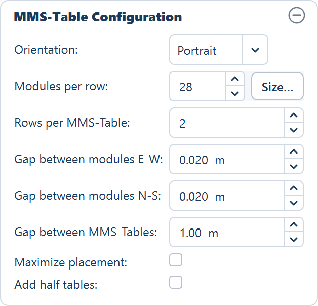
The fields
| Field | Default | Range | What it does |
|---|---|---|---|
| Orientation | Portrait | Portrait or Landscape | Decides which module edge runs east–west and which runs north–south |
| Modules per row | 28 | 1–100 | Modules side by side along one row of the table, east to west. The Size… button beside it opens the string-sizing calculator |
| Rows per MMS-Table | 2 | 1–10 | Rows of modules stacked up the tilted face, north to south. One row is one string |
| Gap between modules E-W | 0.020 m | 0.0–5.0 m | Clear space between neighbouring modules within a row |
| Gap between modules N-S | 0.020 m | 0.0–5.0 m | Clear space between the stacked rows on the same table |
| Gap between MMS-Tables | 1.0 m | 0.0–20.0 m | Clear space east to west, between one table and the next in the same row |
| Maximize placement | off | — | Positions each row of tables independently to hug the boundary |
| Add half tables | off | — | Allows a half-width table where a full one will not fit |
Orientation
Orientation does not rotate the plant. Rows always run east to west and the tilted face always looks toward the equator. What it changes is which edge of the module is the one running along the row.
| Orientation | East–west module dimension | North–south module dimension |
|---|---|---|
| Portrait | The short side | The long side |
| Landscape | The long side | The short side |
Portrait therefore gives a table that is narrow per module and deep up the slope; landscape gives a wide, shallow table for the same module count. Because row pitch is derived from how tall the table stands in its tilt plane, orientation moves the pitch too — see Spacing and tilt.
Table dimensions
The table's two dimensions follow directly from the counts and the gaps:
table width  = modules per row × module E-W dimension
             + (modules per row − 1) × gap between modules E-W

table height = rows per table × module N-S dimension
             + (rows per table − 1) × gap between modules N-S
The gap terms use one fewer than the module count, because gaps sit between modules and not at the ends. Nothing is added for the structure beyond the modules themselves.
A worked example on the defaults
Take the shipped defaults throughout: a 2.38 m by 1.13 m module, Portrait orientation, 28 modules per row, 2 rows per table, and 0.020 m gaps on both axes.
Portrait puts the short side east–west, so the east–west module dimension is 1.13 m and the north–south dimension is 2.38 m.
table width  = 28 × 1.13 + 27 × 0.020
             = 31.64 + 0.54
             = 32.18 m

table height = 2 × 2.38 + 1 × 0.020
             = 4.76 + 0.02
             = 4.78 m
So a default table is 32.18 m across, east to west, and its tilted face measures 4.78 m from the lower edge to the upper edge. It carries 56 modules in two strings of 28. Run your own numbers through the same two lines before trusting a capacity figure — an orientation set the wrong way round is easiest to catch here, at the table, and hardest to catch after the layout has been placed.
The second figure is the length of the tilted face — the collector width — not the footprint it casts on the ground. The footprint is shorter by the cosine of the tilt angle, which is why the row pitch calculation projects it before adding the shading clearance.
Gaps
Three gaps, two of them inside the table and one between tables.
Gap between modules E-W and Gap between modules N-S are the module-to-module clearances the racking needs — clamp space, thermal movement, drainage between rows. Both ship at 0.020 m. They are small numbers that multiply: at 28 modules per row, the east–west gap is applied 27 times.
Gap between MMS-Tables is the clear space left between one table and the next, and ships at 1.0 m. It is east–west only — it separates neighbouring tables within the same row of tables, and nothing else. It is also the figure the cleaning-robot sizing takes as the span of a standard inter-table bridge, so leaving it at a realistic value matters beyond the geometry.
There is no north–south table gap field. North–south separation between one row of tables and the row behind it is the row pitch, derived from tilt and latitude unless you override it. If you are looking for a field to widen the maintenance corridor between rows, it is the pitch override, not a gap.
Rows and strings
One row of modules within a table is one string. Rows per MMS-Table is therefore also the number of strings a full table carries, which is what the inverter or string monitoring box limits are counted against — see Inverter settings.
At the defaults, a table carries two strings of 28 modules. Changing Modules per row changes the string length and so the string voltage; changing Rows per MMS-Table changes how many strings arrive at each combiner. They are not interchangeable ways of adding capacity.
The Size… button
Size…, beside Modules per row, opens the String sizing window, which works out the range of modules in series the module's voltages and the inverter's tracking window allow, and lets you pick a series count and a number of parallel strings. Accepting the pick writes both numbers back here — the series count into Modules per row and the parallel count into Rows per MMS-Table. It needs a module file and an inverter file to be loaded; see String sizing.
What the layout does with the table
Once the table is defined, placement is mechanical. The plant boundary is shrunk inward by the perimeter road width to give the usable area; obstructions, transmission line corridors and terrain exclusions are subtracted from it; and the table is then stamped across what is left, one east–west row of tables at a time.
A table is placed only where it fits entirely inside the usable area. A table overlapping the edge by a centimetre is not placed at all, which is why a large table on a ragged boundary can leave more ground empty than a smaller one would. The two options below exist for exactly that case. Placement itself is covered on How placement works.
Maximize placement
Maximize placement ships off. With it off, tables are placed on a regular grid: every row of tables starts from the same east–west origin, so table columns line up across the whole plant.
Tick it and each row of tables is positioned independently, pushed up against the exact edge of the usable area on that row. On a site with diagonal or curved boundaries this fits extra tables into the wedges a regular grid has to leave empty.
Two consequences to accept before you tick it:
- Table columns will not be vertically aligned across rows. Each row sits where it fits, so the plant reads as staggered rather than gridded. That affects cable runs, road planning and how the drawing looks to a construction team.
- Generation takes longer, and noticeably so on a large site, because each row is fitted on its own rather than stamped from one origin.
Both options are covered together, with the placement behaviour drawn out, on Maximize placement and half tables.
Half tables
Add half tables ships off. A half table is half the east–west width of a full table, carrying half the strings, and it is dropped into any position where a full table will not fit.
- The dimension that halves is the east–west width, and a half table carries half the strings a full table carries.
- Half tables are reported separately in the Summary view, on the Half tables row under Full tables, and count as half a table wherever tables are weighted.
- Nothing is placed anywhere a full table would already have gone. Half tables only ever occupy leftover ground.
- Half tables can also be placed one at a time in Sketch Mode, whatever this option is set to.
Leave it off for a first pass, so the layout you review is the clean grid case. Turn it on when you are chasing the last of the capacity out of an awkward boundary, and check that the resulting fragments are ones your electrical design can actually pick up.
Where to go next
Module specifications
Module dimensions, wattage and bifacial settings on the Array tab, and what loading a manufacturer .PAN file fills in for you.
Tracker configuration
The single-axis tracker unit — geometry, orientation, east–west pitch, rotation limit and the live aperture and ground coverage readout.