Multi-plot sites
One boundary file can hold several separate plant boundaries. Each becomes its own plant, with its own column in the Summary view and its own unit substation.
A boundary file may contain more than one plant boundary. Each one becomes a separate plant: it is laid out on its own, gets its own tables, control rooms, lightning arresters and cables, and gets its own column in the Summary view. This is how a site split by a road, a canal or a change of ownership is designed in one run rather than as several projects.
Nothing about the inputs changes. The module, table, spacing, site and equipment settings apply to every plant in the file, so the plants share a design and differ only in the ground they stand on.
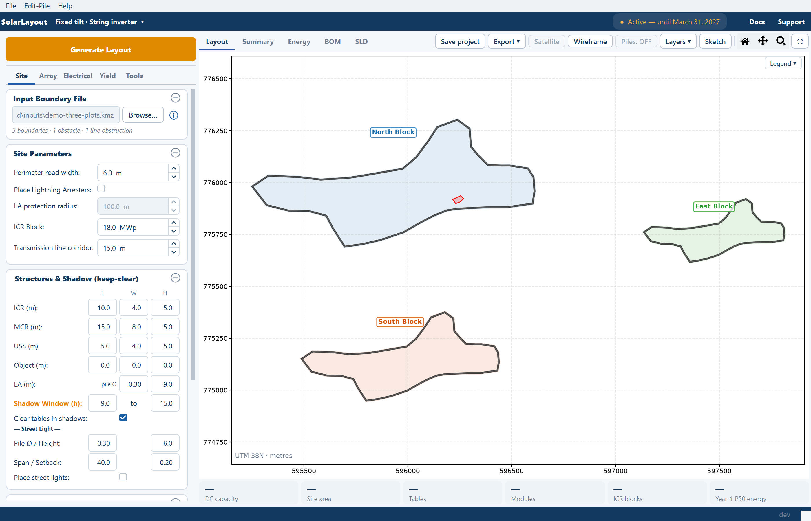
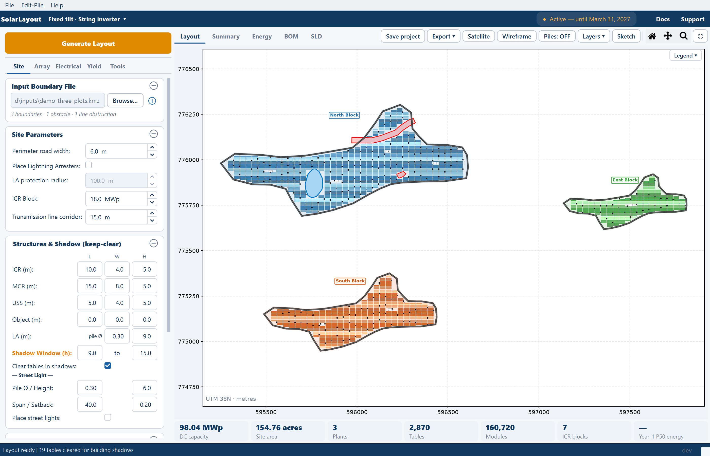
Once a file is read, the line under the boundary field reports how many boundaries it found, and after Generate Layout every plot is laid out in a colour of its own and labelled.
What counts as a plant
The application decides from containment, not from names or from the order features appear in the file:
- A polygon that is not contained within another polygon is a plant boundary.
- A polygon fully contained within a boundary is an obstacle in that plant — a water body, a building, a substation.
So a file with three separate outer polygons produces three plants, and a file with one outer polygon containing three inner ones produces one plant with three obstacles. The difference is entirely whether the polygons are nested.
Each plant is laid out on its own
Every plant runs the whole pipeline for itself. Its boundary is shrunk inward by the perimeter road width to give its own usable area, its own obstructions and corridors are subtracted, its own table grid is placed, and its own control rooms and arresters follow from its own capacity. See How placement works.
Two consequences are worth knowing before you read the numbers:
- The capacity block applies per plant. The number of control rooms is worked out from each plant's own capacity, rounded up — so three plants of modest capacity can carry three rooms between them where one combined plant of the same total capacity would have carried fewer. See Inverter control rooms.
- Every plant gets its own perimeter road. The road band is taken off the inside of each boundary, so splitting one parcel into two plants costs you two road bands instead of one.
What is shared and what is per plant
| Shared across every plant | Worked out separately for each plant |
|---|---|
| The module, table or tracker, spacing and tilt settings | The usable area, and everything subtracted from it |
| The perimeter road width, corridor setback and capacity block values | The road band, the corridors and the number of control rooms those values produce |
| The equipment footprints, shadow window and arrester radius | The placed rooms, arresters, inverters and cable routes |
| The energy assumptions — weather source, losses, degradation, probabilities | The yield figures, because they follow that plant's own capacity |
| The main control room, placed once for the site | The unit substation each other plot receives |
The practical reading of that table: you cannot give one plant a different row pitch, a different table configuration or a different road width. If two parcels genuinely need different designs, design them in separate windows from separate files.
Preparing the file
The rules for a single boundary all still apply, and two more matter only when there are several.
| Requirement | Why |
|---|---|
| Each boundary is a closed polygon — first and last ring coordinate identical | An open ring cannot be shrunk inward or tested for containment |
| Boundaries must not overlap each other | Overlapping outlines make the containment test ambiguous, so a plant may be read as an obstacle in its neighbour |
| Every feature must lie inside the boundary it belongs to | A feature outside every boundary is subtracted from nothing, so tables are placed straight over ground you meant to keep clear |
Full preparation rules, including how each feature must be named for it to be read as water, a canal or a transmission line, are on Boundary file requirements.
If any ring is open, the Check boundaries window lists each problem boundary with a Leave out tick, ticked by default, and a Continue without n button. A boundary left out is not designed at all and does not appear in the Summary view; an unticked one is kept as it is and may produce a wrong layout. Use Fix in Google Earth first and reload the file if you need every plant.
The Summary view gains a column per plant
The Summary view — the second view tab, which replaced the table that used to sit under the plot — turns the figures on their side: a Metric column, then one column per plant, then a Total column that aggregates every plant on the site. The rows are the same for every column, grouped under SITE, ARRAY, ELECTRICAL, CABLES and — once energy has been calculated — ENERGY.
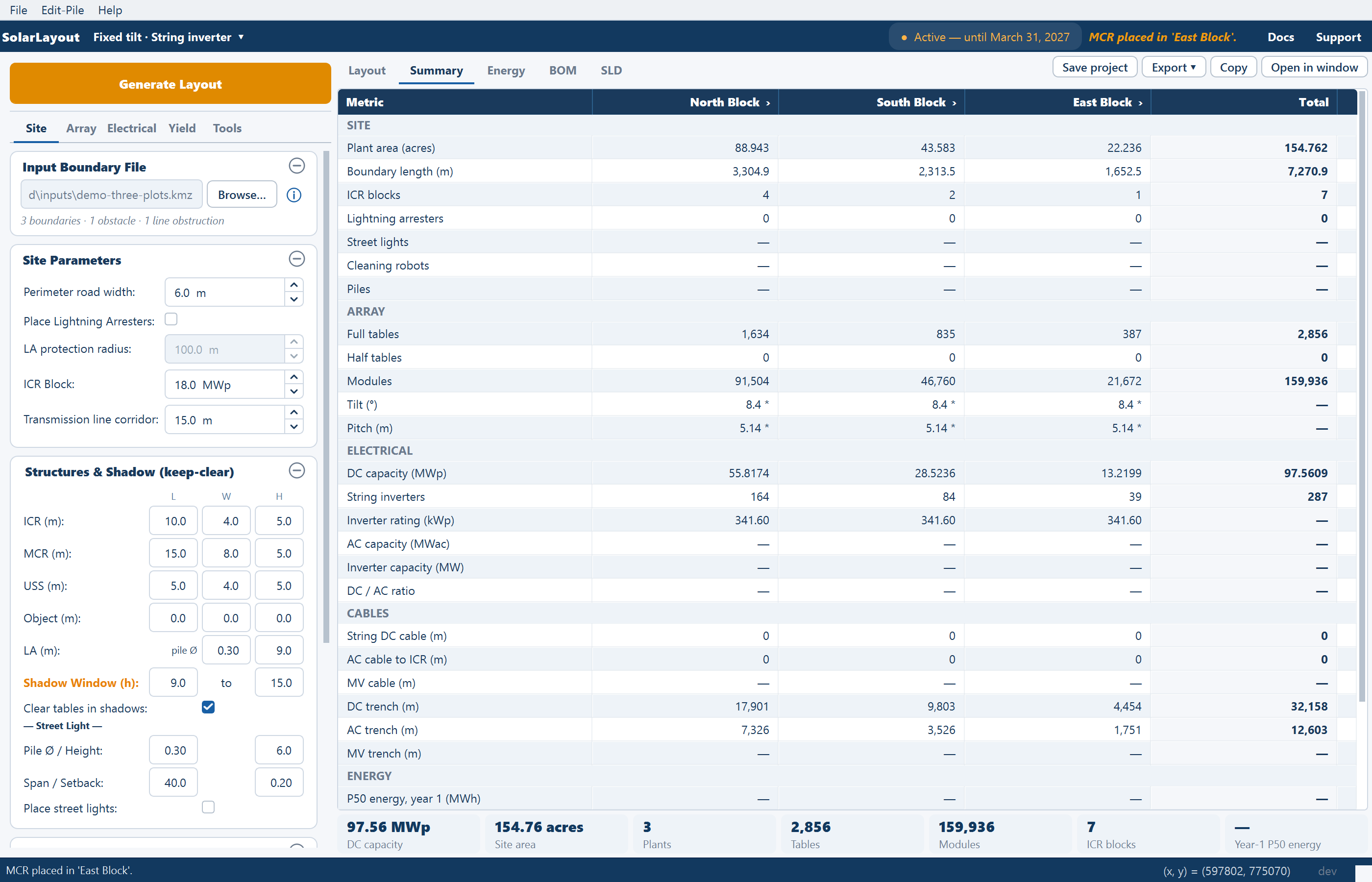
Each plant's column header carries the plant's name with a ›; clicking it shows that plant on the Layout view. Read a multi-plot summary column by column before reading the total. A plant with a poor area-to-capacity ratio is visible immediately next to its neighbours, and it is usually a plant whose shape or corridors are costing it ground. Every row is defined in Summary rows.
With several plants the sheet is wide. Open in window in the view's tools puts it in a window of its own, and Copy puts it on the clipboard as tab-separated text for a spreadsheet.
The Plants chip
The row of plant chips under every view gains a Plants chip on a multi-plot site, carrying the number of plants laid out; the other chips — DC capacity, site area, tables, modules, ICR blocks — are site totals. Water-body results are left out of the totals. Clicking any chip opens the Summary view.

The main control room and unit substations
The main control room (MCR) is placed by hand, once — see Site equipment. On a multi-plot site, placing it does something extra.
Click Place MCR on the Tools tab and the hint reads "n plots — click INSIDE each plot to drop a USS (Unit Substation). The LAST unassigned plot you click gets the MCR. Each plot's ICRs route to its own USS/MCR." Click inside each plot in turn: every plot you click receives a unit substation (USS), and the last plot receives the main control room. Each plot's control rooms then route their medium-voltage cables to the building in their own plot, rather than across open ground to a building in a different plot. That mirrors how the site would actually be built: collection stays inside the parcel it belongs to, and only one circuit leaves each parcel.
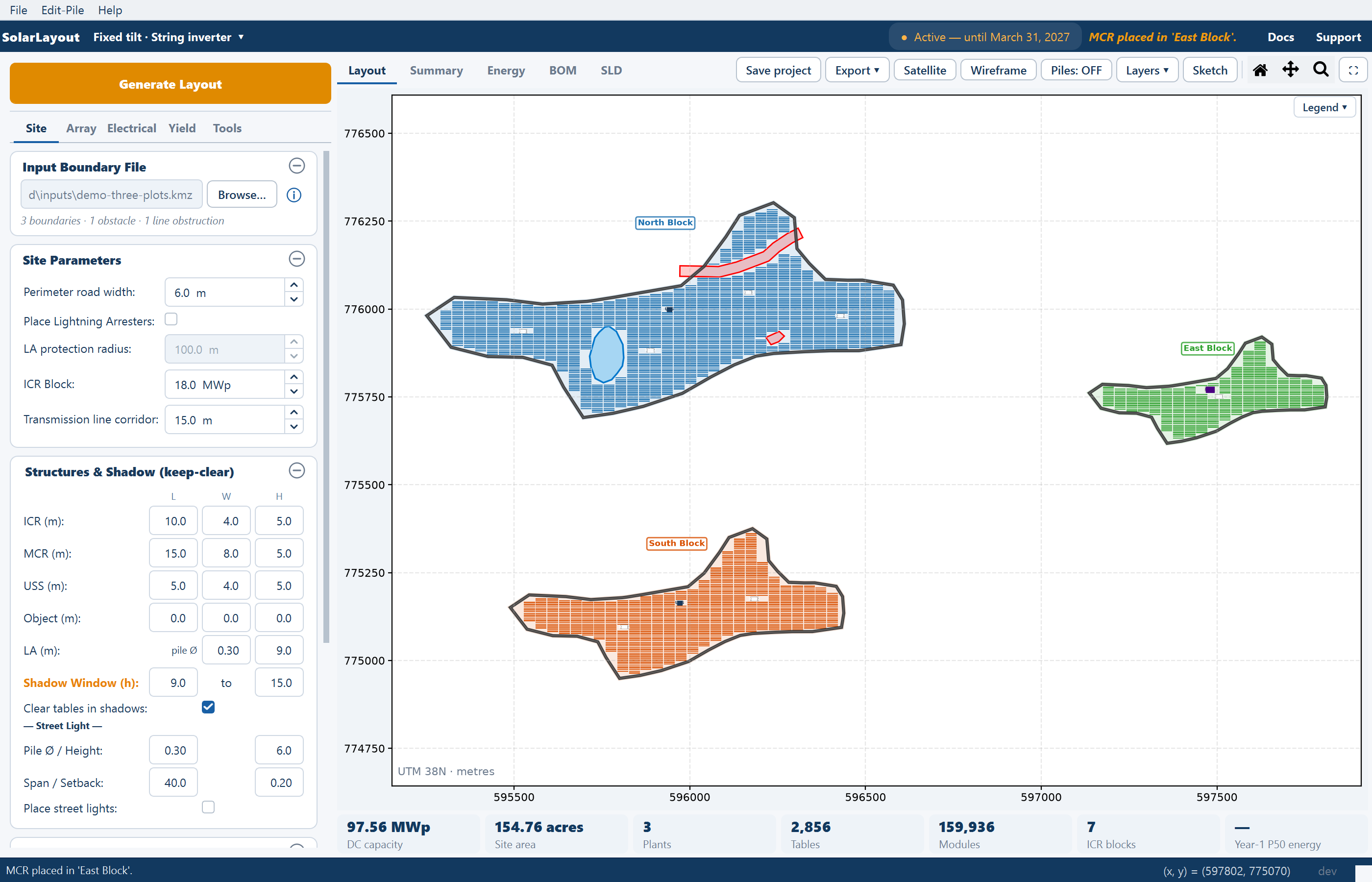
The substation is drawn and cleared at the size set for USS on the Structures & Shadow card, and like every other structure it has a height that casts a shadow. The medium-voltage cables themselves are routed on the next Generate Layout with Calculate cables on, not when the buildings are dropped.
The link that is not routed for you
The connection from each unit substation to the main control room is not part of the automatic routing. It is an overhead line or a buried cable running between parcels, on its own right of way, and it is designed outside the application.
Because that link is not routed, its length is not included in the reported medium-voltage cable lengths. The figures in the Summary view cover the runs from the control rooms to their own plot's substation only. Add the substation-to-main-room lengths yourself before using the cable totals in an estimate.
The routed portion still merges sensibly: within a plot, control rooms whose routes converge share a trunk instead of running parallel lines, so the reported length is a trench-aware figure rather than the sum of straight-line distances. See Cable routing.
What the exports do with several plants
Every export covers the whole site in one file, and each handles the split differently:
- The project report — the Word document from Export ▾ Export Detailed Project Report — draws the site as one drawing and carries the per-plant figures and the total in its design summary, so it is the document to hand over for the site as a whole. See The project report.
- The Google Earth file gets one folder per plant, named after that plant, plus an Overall Summary folder aggregating every plant. That is the export to use when a reviewer wants to look at one plot at a time.
- The CAD drawing has one layer per feature type — boundaries, tables, control rooms, cables — not one layer per plant, so every plant's features share the same layers. See CAD export.
Naming the plants
Each plant appears in the Summary view under the name its boundary carries in the file, and the exported Google Earth file uses the same name for that plant's folder. See Google Earth export.
Name the boundaries for the people who will read the report. Plot A,
Plot B, Plot C is enough to be unambiguous; the parcel or survey numbers
the landowner and the authority use are better, because a reviewer can then
match a summary column to a document without asking you which plot was which.
Rename them in Google Earth before loading the file — the names come from the
file and are not editable in the application.
Reading a multi-plot layout on screen
- Home in the Layout view's tools fits the view to the whole site, every plot included, which is the view to check that no plot was missed. The mouse wheel then zooms at the cursor into any one plot.
- The expand button at the right of the tools gives the drawing its own window — SolarLayout — Expanded View — which is usually necessary before individual plots are legible.
- Satellite is worth a look on a multi-plot site in particular. It shows the ground between the plots — the road, the canal, the neighbouring parcel — and that is where the link between the substations and the main control room will have to run.
Where to go next
Boundary file requirements
Closed rings, containment and the naming rules every feature follows
Summary rows
Every row of the per-plant columns and the Total column
Site equipment
Placing the main control room and the objects around it
Cable routing
What is routed, what is measured, and what is left to you
Cable routing and trenches
How DC, AC and medium-voltage runs are routed, what the conductor and trench totals mean, where they are reported, and how hand-drawn trenches change later runs.
Sketch Mode
The hand-editing surface — select, move, copy, delete, place tables, arresters, roads, corridors and cable trenches on a generated layout, and recompute the plant totals from your edits.